Date: 14 Sep 2013
Author: Colin Broderick
GitHub Repo: github.com/rustyb/cb-tutorials
QGIS Tutorial
The aim of this tutorial is to demonstrate the application of three common tools present in any GIS system.
The tutorial provides step by step instructions to be followed in order to complete the tasks.
Quicklinks
Goals | Software | Data | Prepare Map | Load Data | Query the data we want | Identify Features | Load Transport Data | Basic Statistics | Buffers | Intersect | Area Calulation
Goals
- Understand how to load shapefiles QGIS and perform some basic geosptaial analysis.
- Create spatial query data to display only the required features and export that as a new shapefile reprojected.
- Using the buffer tool - know how to create them and use to assess potential catchments.
- Use the intersect tool to extract the area of a polygon covered by a buffer and identify the area of this new polygon.
Software
- QGIS 1.8.0 - Lisboa
Tutorial Data
Census Data
CSO Census Boundary links census.cso.ie/censusasp/saps/boundaries/ED_SA%20Disclaimer1.htm
SAPS Boundaries - http://census.cso.ie/censusasp/saps/boundaries/Census2011_Small_Areas_generalised20m.zip Projected is ING = TM65 / Irish Grid - EPSG Projection 29902
You will need to agree to the terms of use to obtain this data.
LUAS Data:
- Luas Line Alignments and Stations (Dublinked) dublinked.com/datastore/datasets/dataset-301.php
- download the zip file and unzip
Download and Unzip all the data
Prepare your map
Open QGIS
You will now be presented with a new map project. It is a good idea to save this map project for future use.
So first thing we will do is click File - Save Project
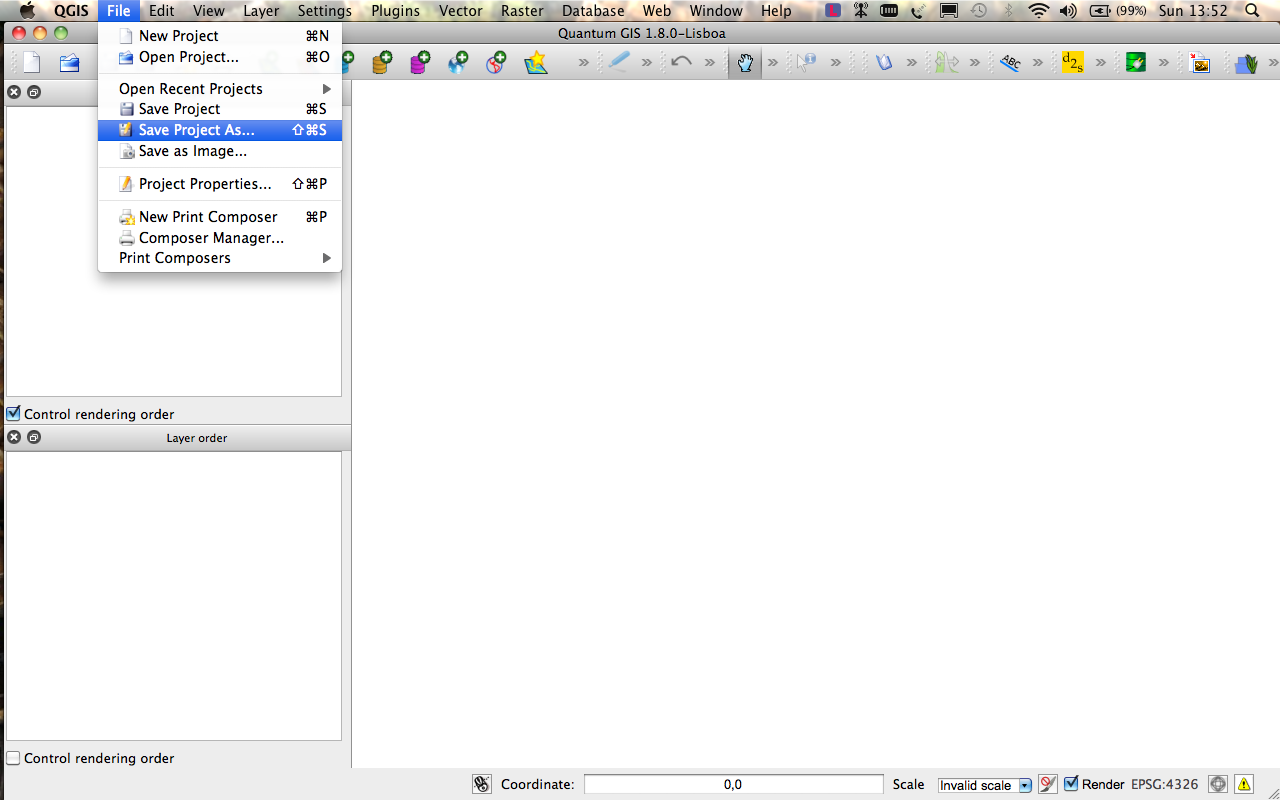
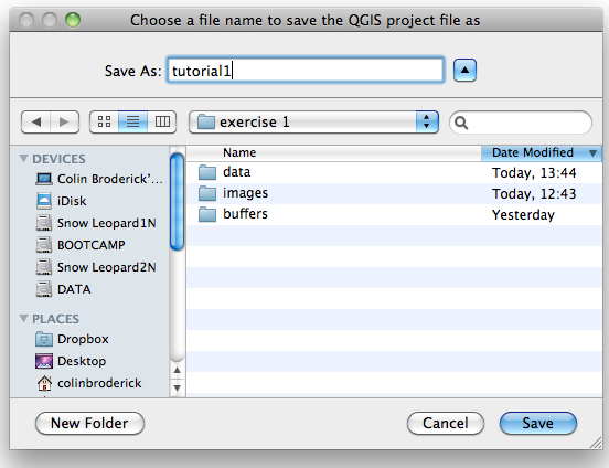
Give your project file a meaningful name, it is advised that you save the project in the same folder as you have your lab data.
Next we know that our data is projected in Irish Grid (TM65) from the census and we know that our light rail data is in Irish Transverse Mercator we will set the coordinate projection system of our project to ITM.
You can do this two different ways.
1 Click File -> Project Properties or (SHIFT + CMD + P)
2 Click the co-ordinate system tab
3 Check enable on the fly CRS projection
4 Search for ESPG 2157
5 Select it and click apply.
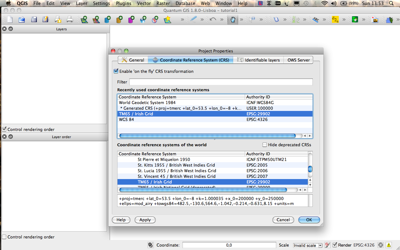
6 Save your project.
Setting on the fly crs projection will allow us ot view the datasets with different projections re-projected to a single projection so they display correctly.
OR
Click the little globe in the bottom right hand corner of your screen and then follow steps 3 - 7 above.
Load your lab data
1 You should have already unzipped the census SAPS areas file by now, if not please do this now.
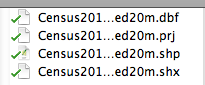
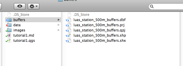
2 You should have a folder with a shapefile, a dbf, projection and shx file.
3 Click the Add Vector Layer icon in the top bar.

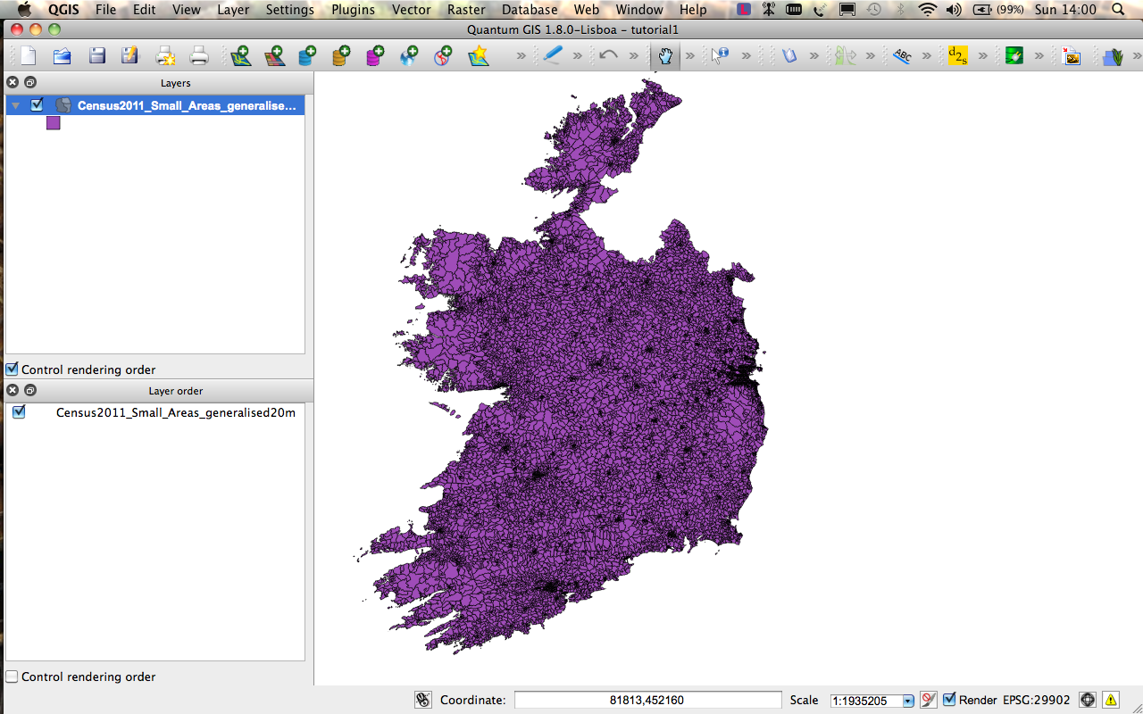
4 Browse to your file and load the .shp file.
5 You should then be presented with a view like so:
Query the data we are interested in
For the purposes of this tutorial which is find out how many people might be living within 500m of the two light rail lines in Dublin we only care about the data in the county of Dublin.
The county of Dublin is spilt into 4 local administrative areas or local authorities (county councils) and for the purposes of the census these administrative areas are party of the Dublin NUTS3 area.
So lets find out how to query our data to only show the Dublin Region.
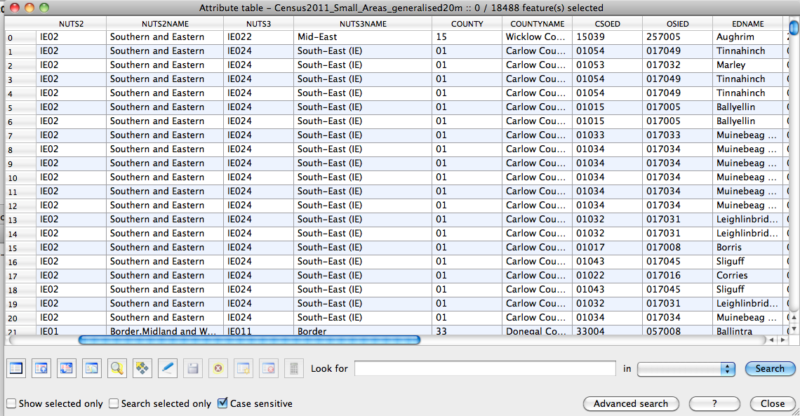
1 Open your attribute table by right clicking on the layer and selecting attribute table. A window will open like below:
 [image for attribute table]
2 If you scroll across you can see the two columns we are interested in NUTS3 and NUTS3NAME.
3 Next we want to only show the rows that have Dublin as their NUTS3NAME.
4 Right click the layer and click Query.
5 You will see a query window like this that allows you to construct spatial queries in an SQL style query format.
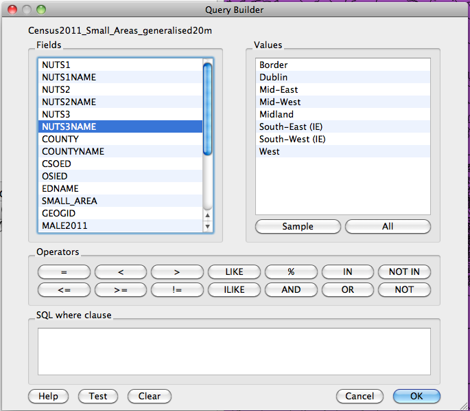
6 Highlight the NUTS3NAME column and click All on the right.
7 You are now presented with all the values in this Column. There are only 8 unique values in this column so clicking sample gives the same result. If you know there are is a large number of values in a column you should click sample to see a few of them as clicking all may take some time to load as the query builder has to read all the values associated with that field which could be in the 1000's.
8 We are going to construct a very simple query here which is as follows:
"NUTS3NAME" = 'Dublin'
9 To do this double click NUTS3NAME it will be inserted into the Query Window.
10 Click the = operator.
11 Double click Dublin and it will be inserted into the query window after the =
12 If you have used the right syntax when you click test you will receive an answer like below:
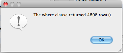
14 If this is your result congrats you have run your first spatial query successfully!
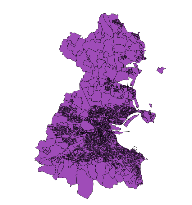
15 We now need to save this data to a shapefile with the same projection as the luas data Irish Transverse Mercator. To do this right click the layer and click save as. Save this file with the filename Census2011_Small_Areas_generalised20m_dublinITM. This will enable us to only run analysis and statistics between the two layers.
Census2011_Small_Areas_generalised20m_dublinITM
Lets find out more about the data
1 To see the attribute of a single polygon (SAPS Area). Click the Identify Features tool.

2 Click one of the polygons on the map. In my case I picked Small_Area 267005001 which is located in the Electoral District of Balgriffin. It had a total population in 2011 of TOTAL20113 = 636 people.
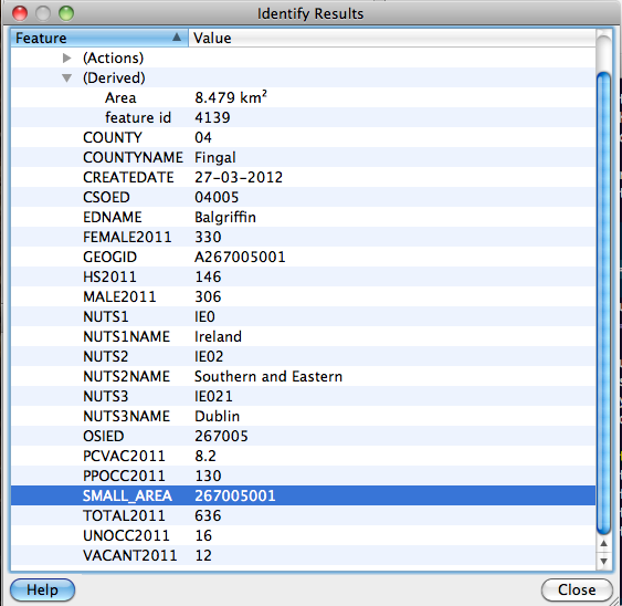
3 Other information within the identify features dialogue which are derived using the current co-ordinate system is the features area in this case 8.479 km squared.
4 That's all very interesting but say we wanted to drill down more and we wanted to see all the small areas in dublin that had a population of 500 or more people on census night we can do that easily.
5 Open the Query window. We already have our query restricted to only small areas in Dublin.
"NUTS3NAME" = 'Dublin'
6 We will now add an AND to add another statement to this.
7 We are looking for total population so we insert "TOTAL2011" followed by >= (greater than or equal to) 500
"NUTS3NAME" = 'Dublin' AND "TOTAL2011" >= 500
8 Click test and if your syntax is correct you should have 51 rows.
9 Click Ok the result should look like this:

10 Now go back to the query window and remove the AND "TOTAL2011" >= 500 statement to return to showing all small areas in Dublin.
Load your Transport DATA
Ok now that everything is using ITM and we have turned off on the fly CRS transformation we are sure each layer is in the right place.
Load the shapefiles as before:
- Luas_Network_2012_Alignment_ITM.shp
- Luas_Network_2012_Stops_ITM.shp
You should have two new lines and a number of points which represent the stations or stops on the LUAS Lines (LRT).
Ok so now we can do some very simple selections of small areas. Say we as a transport planner wanted to see all the Small Areas that the LUAS lines cross.
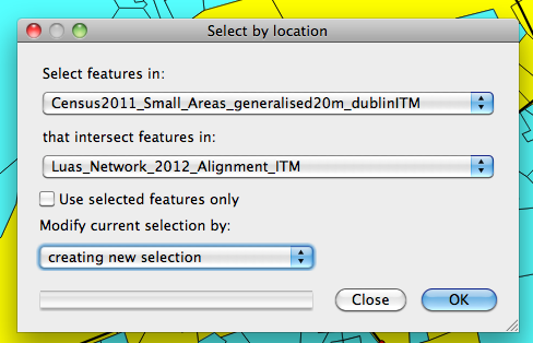
1 First go to Vector in the top bar and scroll down to research tools -> Select by Location.
2 Select the Dublin Census layer
Basic Statistics
Now say we would like to find out the total population in those areas on Census night. We can do this easily using the Basic Statistics Tool.
1 Click Vector -> Analysis Tools -> Basic Statistics
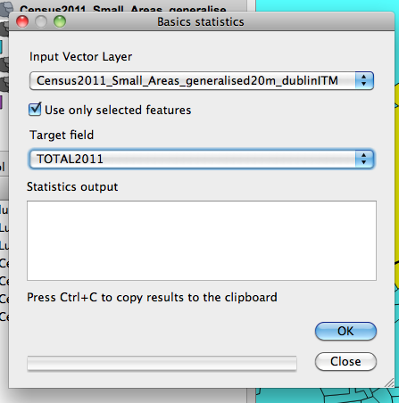
2 Select the Dublin Census Layer.
3 Make sure use only selected features is checked.
4 For our Target Field we select TOTAL2011
5 Click ok and you will get an output like you will see below:
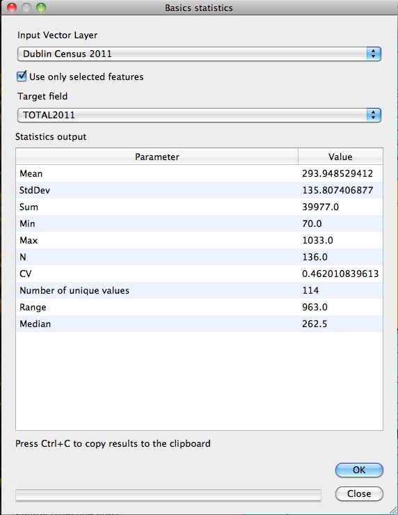
6 As you can see the total population within areas that the line passes through is a sum of 39977 people.
7 To compare maybe could select only those areas that a station is located within.
8 Go to Select by Location and this time create a new selection with features in Dublin Census 2011 that intersect with features in Luas Stops or Stations.
9 We have selected only 49 features this time.
10 Go to basic statistics and run the same query again on the new selection.
11 This time the total population is 16745 people
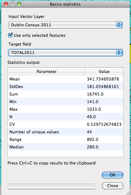
That's roughly half the people that are located along the alignment. But as a transport planner we know that the catchment from a transit stop is usually 5mins walk distance or else 500m. So now we would like to find all the areas located within 500m of the LUAS stops.
Buffer
To do this we will use a buffer.
The buffer tool creates a 500m area surrounding each feature in the layer such as a point, line or polygon.
1 Vector -> Geoprocessing Tools -> Buffer(s)
2 Select Luas Station Stops
3 Uncheck use only selected features
4 For buffer distance enter 500 - we know that the base unit used in ITM is the meter so this will create a 500m buffer.
5 Select a location for the shapefile that will be created containing the buffers. I put mine in a specific buffers folder in my exercises folder as below:
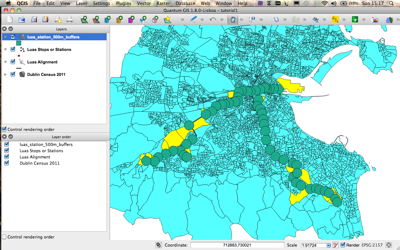
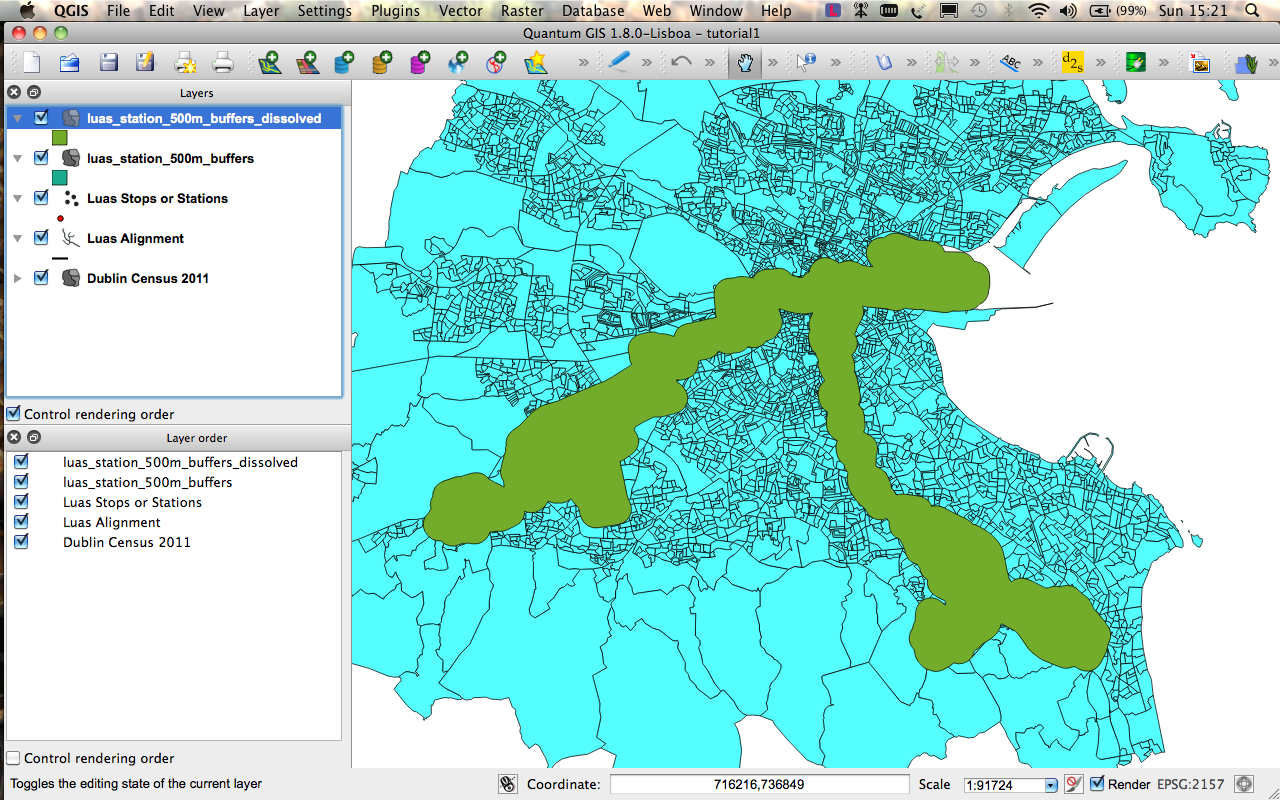
6 The results of the buffer are below. you can see that some of the polygons created overlap. If you check the option Dissolve buffer results when creating the buffers it will merge all the buffers and connect them up as you can see below:
Regular Buffers
Dissolved Buffers
7 Now run the statistics on this new selection and your result should be a total of 184,128 people
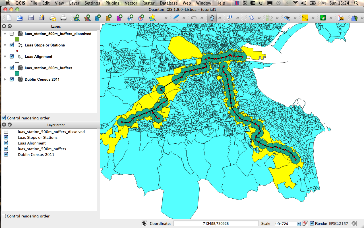
This method has limitations as using this selection method the buffer only has to intersect with the small area at any point and then it will be selected.
Furthermore we do not know the distribution of people across the census small area nor do we take account of the how large or small a portion of the census are the buffer covers so we cannot say for sure that the potential catchment is 184,128 people.
Intersect the buffers with the polygons and find the area
The next and final piece of this tutorial will be to cut out the section of the small areas covered by the buffers and then to calculate the area of these new polygons.
To do this we use the Intersect Tool 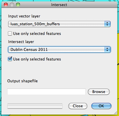
Intersect
1 Click Vector -> Geoprocessing Tools -> Intersect
2 Select the Buffers layer as your input layer and Dublin Census 2011 as your target layer.
3 Make sure to check Use only selected features as the polygons intersected by the buffers should still be your current selection.
4 Pick a location for the new shapefile. Click Ok.
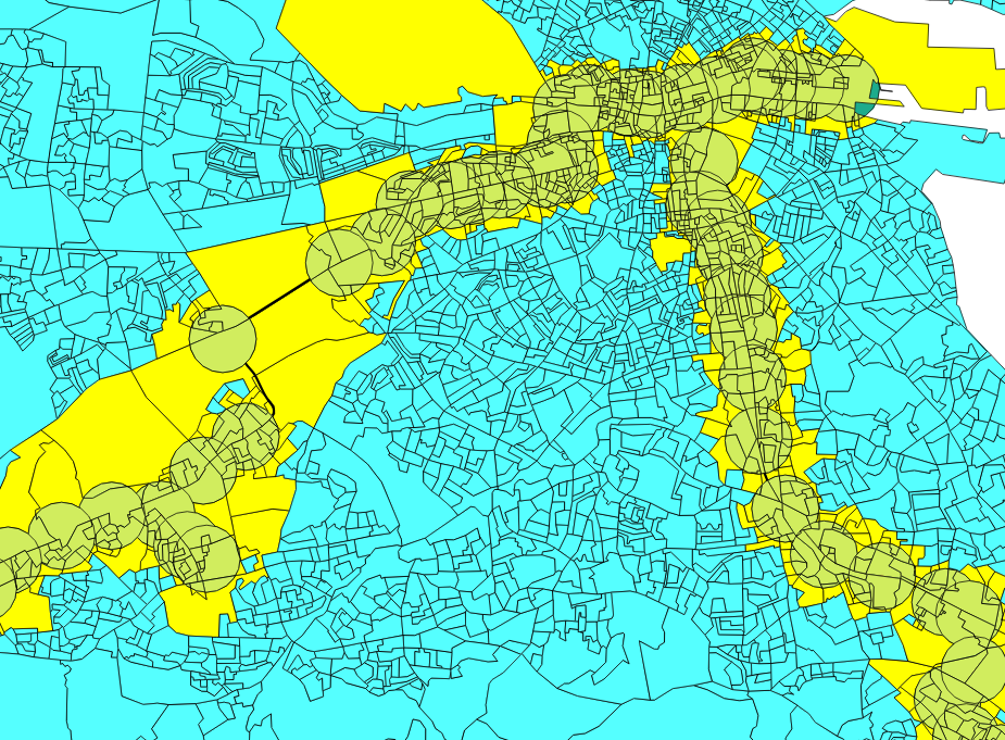
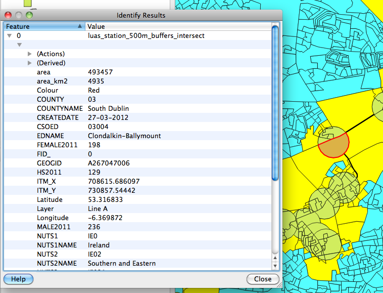
5 Add this new layer to your map.
It should now look like this:
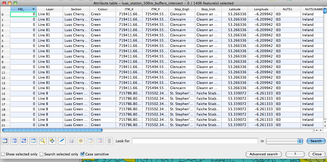
6 Now right click on this layer and go to the attribute table. You will see that the new shapefile contains the attributes from both the input and target layer.
Area Calculation
1 Now we are going to calculate the area. Click the edit icon  and click the field calculator
  .
.
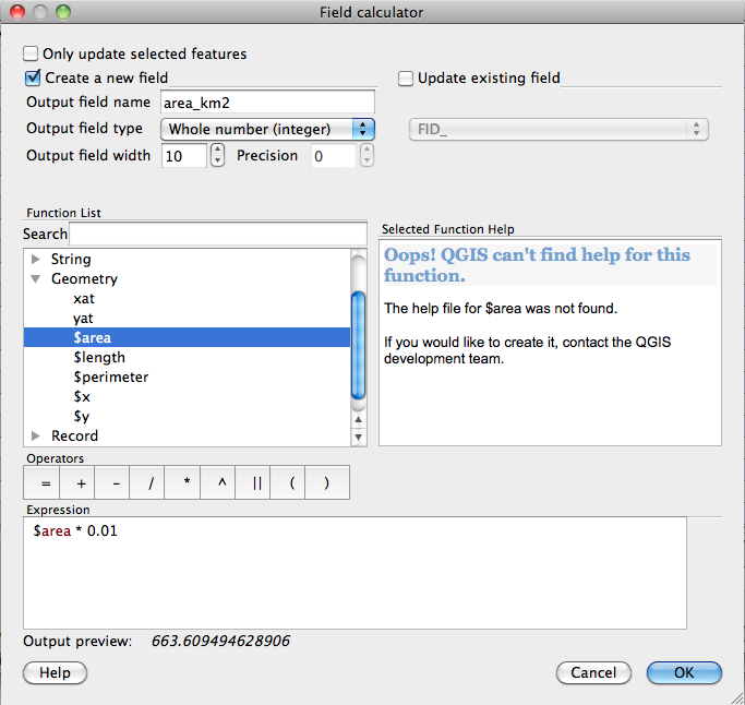
2 Now we want to add a new field to calculate the square km size of the shape. So make sure to check Create new field.
3 Enter the field name as
area_km2
4 Scroll down to geometry and double click $area
We know that a hectare is 0.01 of a square kilometer so we need to multiply the answer as it will be in hectares by 0.01.
Your query should be as follows:
$area * 0.01
6 Now click ok and you will see the new field at the end of the table.
7 Click save and click the edit button once more to exit editing mode.
8 Now save your project.
9 Congratulations you can now calculate the area of a shape using the field calculator.
This will be used in the next tutorial to help you calculate the fraction of the area of the total polygon (small area) covered by the buffer and find out the population if we assumed the population was evenly distributed across the area.